At time of writing, SAP Analytics Cloud (Q4, 2021.20) does offer dynamic calendar-based time filtering. This enables users to quickly analyse data for periods such as Current Year, Quarter and Month to Date. The same functionality is also exposed when working with SAP BW Live models containing a 0CALDAY dimension.
The limitation is that for BW Live models, the platform has no awareness of Fiscal / Financial periods. SAC offers no native mechanism to dynamically present common reporting scenarios such as Financial Year to Date, or even just Current Financial Year. All dynamic options Calendar based only.
The Requirement
My organisation needed a solution which allowed Self Service users a way to easily build Stories which rely heavily on Financial Year time periods (July – June FY in Australia). The solution had to be:
◉ As simple as possible for end users to understand and use
◉ Flexible, so that users could define their own dynamic ranges (we couldn’t predict every scenario, so proliferating measures in models was not viable)
◉ Dynamic, so that users would not need to manually update filters in Stories as time moved on
◉ Rapid to implement from a development perspective
◉ Low maintenance from a BW perspective – no additional staging of data or loads
◉ Easy to roll out to all relevant existing Composite Providers and queries.
Below I describe an architected solution enabling users to create dynamic Restricted Measures or just add dynamic time filtering to Stories in SAC.
Step 1: Establishing the Building blocks
To start off, I first needed to address another age-old limitation which is that the delivered BW time characteristics cannot have custom attributes added to their master data. The solution here was simply to create two new standard InfoObjects which would carry the attributes that could not be added natively to 0FISCYEAR and 0FISCPER3.
◉ Two new InfoObjects are created in BW, named FISCYEAR and FISCPER3.
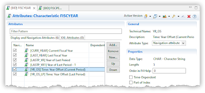
FISCYEAR is created as NUMC(4), with Master Data and also Texts (optional) selected:
Six attributes are then added. The first four are a simple flag and so are typed as CHAR(1). The last two are CHAR(5) to contain some offset values which will be calculated. All are marked as Navigational.
Not all of these are critical for the solution, in fact only the last two will be exposed to SAC later in the demo. The other flags we have in use for specific unrelated modelling requirements.
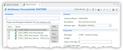
FISCPER3 is created as CHAR(3) to mimic 0FISCPER3. It just has Master Data defined.
Four attributes are defined, in this case all are CHAR(1) just containing a flag.
Step 2: Adding the Master Data
In order to provide dynamic master data to these new objects without requiring any additional data loads or persistence, a choice was made to provide virtualised master data sourced from a HANA View.
We can natively read an SAP HANA Calculation View to provide master data for an InfoObject, but in this situation I wanted to script the logic so began with two Table Functions which were then exposed through Calculation views.
SAP HANA Table Functions
The Table Function for FISCYEAR master data provides a generated list of Financial years, determining all the required attributes in addition to the Display Text used in other reporting:
FUNCTION "_SYS_BIC"."ZBW.Functions::TF_FISCYEAR_MASTER" ( )
RETURNS TABLE ( FISCYEAR VARCHAR(4),
CURR_YEAR VARCHAR(1),
LAST_YEAR VARCHAR(1),
CURR_YEAR_LP VARCHAR(1),
LAST_YEAR_LP VARCHAR(1),
YEAR_OFFSET VARCHAR(5),
YEAR_OFFSET_LP VARCHAR(5),
TXTSH VARCHAR(20))
LANGUAGE SQLSCRIPT
SQL SECURITY INVOKER
DEFAULT SCHEMA SAPHBW AS
BEGIN
DECLARE CURR_YR INT = YEAR(CURRENT_DATE);
DECLARE CURR_YR_LP INT = YEAR(ADD_MONTHS(CURRENT_DATE,-1));
IF MONTH(CURRENT_DATE) > 6
THEN CURR_YR = CURR_YR + 1;
END IF;
IF MONTH(ADD_MONTHS(CURRENT_DATE,-1)) > 6
THEN CURR_YR_LP = CURR_YR_LP + 1;
END IF;
RETURN
SELECT
ABAP_NUMC(GENERATED_PERIOD_START, 4) AS FISCYEAR,
CASE GENERATED_PERIOD_START
WHEN :CURR_YR THEN 'X' ELSE ''
END AS CURR_YEAR,
CASE GENERATED_PERIOD_START
WHEN :CURR_YR - 1 THEN 'X' ELSE ''
END AS LAST_YEAR,
CASE GENERATED_PERIOD_START
WHEN :CURR_YR_LP THEN 'X' ELSE ''
END AS CURR_YEAR_LP,
CASE GENERATED_PERIOD_START
WHEN :CURR_YR_LP - 1 THEN 'X' ELSE ''
END AS LAST_YEAR_LP,
CASE
WHEN GENERATED_PERIOD_START - :CURR_YR = 1 THEN 'NEXT'
WHEN GENERATED_PERIOD_START - :CURR_YR = 0 THEN 'CURR'
WHEN GENERATED_PERIOD_START - :CURR_YR = -1 THEN 'LAST'
WHEN GENERATED_PERIOD_START - :CURR_YR < -1 THEN '-' ||
ABAP_NUMC(GENERATED_PERIOD_START - :CURR_YR,2)
ELSE ABAP_NUMC(GENERATED_PERIOD_START - :CURR_YR,2)
END AS YEAR_OFFSET,
CASE
WHEN GENERATED_PERIOD_START - :CURR_YR_LP = 1 THEN 'NEXT'
WHEN GENERATED_PERIOD_START - :CURR_YR_LP = 0 THEN 'CURR'
WHEN GENERATED_PERIOD_START - :CURR_YR_LP = -1 THEN 'LAST'
WHEN GENERATED_PERIOD_START - :CURR_YR_LP < -1 THEN '-' ||
ABAP_NUMC(GENERATED_PERIOD_START - :CURR_YR_LP,2)
ELSE ABAP_NUMC(GENERATED_PERIOD_START - :CURR_YR_LP,2)
END AS YEAR_OFFSET_LP,
ABAP_NUMC(GENERATED_PERIOD_START - 1, 4) || '/' ||
ABAP_NUMC(GENERATED_PERIOD_START,2) AS TXTSH
FROM "PUBLIC"."SERIES_GENERATE_INTEGER" (1, 1970, 2100);
END;
The above function returns several flags based on the determination of the current Financial Year, derived from the current system date.
It also calculates offset values from the Current Determined Financial Year which are the ones critical to this solution.
You will notice two variations in the flags and offsets determined above. One set will support reporting where the user needs to include derivation from the current open Month, and the second set calculate values based on the last Period.
Within my organisation most financial reporting takes place against completed periods, so the current open period is generally excluded. Some reporting requirements however do need to reference the current month. Providing both sets allows flexibility for end users while building their SAC Stories.
It is worth noting that the above code assumes the Australian Financial Year, beginning in July and ending June the following calendar year. Within my organisation we do not have a requirement to support international reporting for different Financial Year Variants. If there was a requirement to do so, then the likely approach would be to compound FISCYEAR against 0FISCVAR as per standard BW, and enhance the code above to provide determinations for the different Fiscal Year Variants.
Noting also that this function leverages SERIES_GENERATE_INTEGER to provide a generated input list of Years. I chose to provision data for a range of 1970 – 2100. This range could be enlarged or reduced by updating the parameters, or even dynamically determined using the current year to provide a sliding window.
For the ‘Year Offset’ values, I chose to provide unique text values for the Current, Next and Last Financial Years to improve the SAC user experience, but these could be omitted and just left as numerical values depending on preference.
The function outputs a list of values similar to the following:
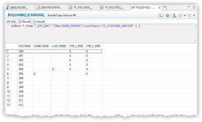
The Table Function for FISCPER3 master data provides a generated list of Financial Periods from 000 – 012, determining all the required attributes for both contexts of based on current open period, or last completed period.
FUNCTION "_SYS_BIC"."ZBW.Functions::TF_FISCPER3_MASTER" ( )
RETURNS TABLE ( FISCPER3 NVARCHAR(3),
CURR_PERD NVARCHAR(1),
LAST_PERD NVARCHAR(1),
YTD_L_PER NVARCHAR(1),
YTD_C_PER NVARCHAR(1))
LANGUAGE SQLSCRIPT
SQL SECURITY INVOKER
DEFAULT SCHEMA SAPHBW AS
BEGIN
-- Generate initial list of periods using SERIES_GENERATE_DATE
-- The years of the dates passed to SERIES_GENERATE_DATE are not critical as we just need one record for the 1st of each month
-- Initial DUMMY SELECT starts table with record for period '000'
-- Current and Last Period flags derived from current system date, so are calendar based
PeriodTab =
SELECT '000' FISCPER3,'' CURR_PERD,'' LAST_PERD FROM DUMMY
UNION
SELECT
ABAP_NUMC(ELEMENT_NUMBER,3) FISCPER3,
CASE WHEN MONTH(GENERATED_PERIOD_START) = MONTH(CURRENT_DATE) THEN 'X' ELSE '' END CURR_PERD,
CASE WHEN MONTH(GENERATED_PERIOD_START) = MONTH(ADD_MONTHS(CURRENT_DATE,-1)) THEN 'X' ELSE '' END LAST_PERD
FROM SERIES_GENERATE_DATE('INTERVAL 1 MONTH', '2000-07-01', '2001-07-01');
-- Return statement uses initial generated table plus two extra columns derived for the Current and Last Period
-- The inline nested SELECT statements look inefficient but performance is actually better than assigning Scalars up front
RETURN
SELECT
FISCPER3,
CURR_PERD,
LAST_PERD,
CASE WHEN FISCPER3 <= (SELECT FISCPER3 FROM :PeriodTab WHERE LAST_PERD = 'X') THEN 'X' ELSE '' END AS YTD_L_PER,
CASE WHEN FISCPER3 <= (SELECT FISCPER3 FROM :PeriodTab WHERE CURR_PERD = 'X') THEN 'X' ELSE '' END AS YTD_C_PER
FROM :PeriodTab;
END;
SERIES_GENERATE_DATE is used to supply a source list of dates which are processed for the attributes. The generation start and end Years are not important as long as the months align with the start and end months for the required Financial Year construct.
Again if you needed to support multiple fiscal year variants then the object could be compounded to 0FISCVAR and the function updated accordingly.
The function outputs a list of values similar to the following:
Graphical Calculation Views
Now that we have the two HANA Table Functions in place, two graphical Calculation Views are created to just present the output directly. Since there is no additional logic contained in the Calculation views, I have not included additional detail for these. They are configured with a Data Category of ‘Dimension, and just use a single Projection node to map all the Table Function fields to the Semantics.
Populating the Master Data
Mapping the output of the Calc Views to the InfoObjects is performed via configuration of the Read Access for the InfoObjects on the Master Data/Texts tab for the InfoObjects.
The results are now visible in the Master Data view for the InfoObjects:
Step 3: Adding Dimensions to the Composite Provider
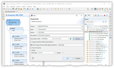
With the new InfoObjects now available, they need to be added in to the Composite Providers as required. This can be done just with a field mapping in the Target scenario
Once the target fields are created and associated with the new InfoObjects, then the existing source fields for 0FISCYEAR and 0FISCPER3 can be directly assigned.
In the Output tab, all Navigation Attributes are then enabled for both FISCYEAR and FISCPER3.
With the Navigational Attributes now available in the Composite Provider, they can be added directly to any Queries used as BW Live data models in SAC. The new Nav Attributes will then become available as dimensions within the Live BW Model.
Using the new Dimensions
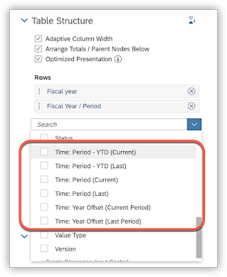
In their simplest form the new dimensions can be directly added to any Story in SAC. The example below is for illustration purposes to see how the dynamic dimensions come through.
Note that for the flag based dimensions, short texts have been maintained in BW just for presentation purposes.
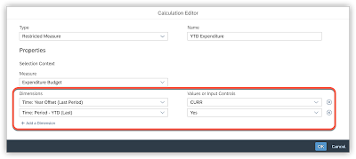
Probably the main purpose for the new Dimensions however would be to create dynamic Restricted Measures for use in charting and reporting. The benefit being that as time moves forward, the parameters for the Restricted Measures do not need to be updated as the values in the Dimensions will change according to the date.
For example, creating a Restricted Measure for YTD Budget values (not including the Current Period):
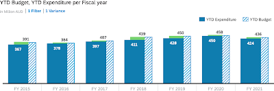
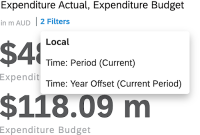
Because the Period flags have been added to FISCPER3 rather than FISCPER, it is generally necessary to restrict on the Fiscal Year dimension also to avoid a selection spanning multiple years. However in some situations this also may be useful. For example, in the figure below the Financial Year filter has been intentionally omitted from the Restricted Measures. Instead, a breakdown by Year is performed indicating the year on year performance against budget for the same YTD time frame. Here a filter is applied at the Widget level, selecting the LAST, -02, -03, -04, -05, -06 & -07 relative years. This time window would also increment dynamically as the years rolled over.








No comments:
Post a Comment