The actual solution of the question above is super-easy and comes down to a single select statement using a spatial join. So, the major part of this explanation will be about data import of the following files:
1. We need a dataset with global latitude and longitude data. On Kaggle there is a nice data set with Global Power Plants. This dataset already contains a country column, which we will of course ignore (otherwise the question above does not make much sense). Instead of this, you can also use your own dataset, where the problem statement makes more sense.
2. To determine to which country a coordinate belongs, we need to have an idea of the extent of each country. The easiest way is to upload a shapefile with global country borders to our SAP HANA Cloud database.
Import a CSV file with Latitude and Longitude Values
The first part is not even related to the initial question, since you would typically already have some lat/lon data in your database when asking this question. Still, I think it’s a good idea to make the upload part of the description, so that this blogs works as a self-contained end-to-end example.
Please skip this part in case you want to leverage your own lat/lon dataset.
1. Download and unzip the Global Power Plants dataset from Kaggle (requires a free account).
2. Open your SAP HANA Cloud instance in Database Explorer
3. Right-click your instance and choose ‘Import Data’
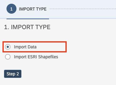
4. Choose ‘Import Data’ again
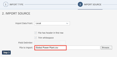
5. Select the downloaded CSV file
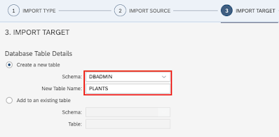
6. Choose your import target
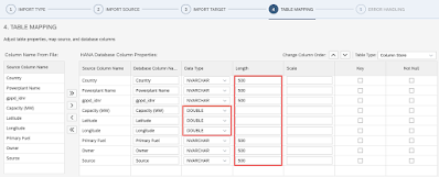
7. Adjust the type mapping. Make sure to change Capacity, Latitude and Longitude to Double and increase the length of the text types (e.g. to 500).
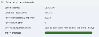
8. Start the import and wait for the records to be imported into table ‘PLANTS’.
You wouldn’t believe it, but this was the most complex part! From now on, things will get easier.
Import a Shapefile with Global Country Borders
Next, we need to import the global country borders. The easiest way to do this is by using a standard exchange format for spatial data – the so called
Shapefile.
2. Do not unzip this file. The zip format is just fine for import.
3. As before, open Database Explorer, right-click your instance and choose ‘Import Data’.
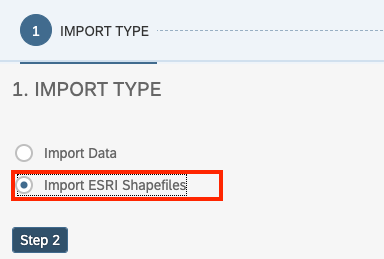
4. This time select ‘Import Esri Shapefiles’
5. Select the downloaded zip file
6. Select the target schema for the import. I am using the same target as for the CSV import.
7. As a Spatial Reference Identifier choose “WGS 84 (planar)” with SRID 1000004326.
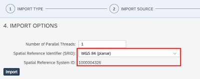
8. Start the import and wait for the records to be imported into table ‘world-administrative-boundaries’.
We have now imported all the data for our example.
Determine the Country for each Power Plant
Again, our power plant dataset already has the country information included. We will ignore this information and add the country by the knowledge of latitude and longitude information. Of course, we can use the country information of the dataset itself to double-check our results for correctness.
To match each lat/lon point with its country, we need to execute two spatial operations:
1. Create a point geometry from lat/lon information. This can be done using SQL function
ST_GeomFromText. The minimal usage example looks like the following:
SELECT ST_GeomFromText('POINT(8.642057 49.293432)', 1000004326) FROM DUMMY;
2. We do a spatial join by predicate
ST_Intersects to match two entries in the respective table in case the point is contained within the polygon of the country.
Knowing these two spatial functions, we can add the country information from table ‘world-administrative-boundaries’ to our data table by executing this SQL query:
SELECT wab."iso3", wab."name", p.*
FROM PLANTS p
LEFT JOIN "world-administrative-boundaries" wab
ON ST_GeomFromText('POINT(' || p."Longitude" || ' ' || p."Latitude" || ')', 1000004326).ST_Intersects(wab.SHAPE) = 1
As a result we added columns “iso3” (the ISO code of the country) as well as the standardized “name” to our result set. We can also see that the information matches the datasets country in most cases. Exception can be found in the bordering regions of countries, where the level of detail of the used world border are probably not sufficient.

This solved our initial question. So everyone, who is short on time, can safely stop reading.
⚠️ In this example we are generating the geometries on the fly instead of using the built-in column type ST_Geometry. Thus SAP HANA cannot make use of spatial indices, which results in decreased performance. I strongly recommend to use persistent geometries with type ST_Geometry for productive scenarios.
Add Additional Insights By Spatial Aggregation
Now, that we already have the data imported and sufficiently answered our initial question, we may as well add a little analysis on top. The following view helps us identify the countries with the most capacity by power plants. Note, that we aggregate over the spatial dimension.
CREATE OR REPLACE VIEW CAPA_PER_COUNTRY AS (
SELECT wab."iso3", wab."name", wab.SHAPE, SUM(p."Capacity (MW)") AS CAPACITY
FROM PLANTS p
JOIN "world-administrative-boundaries" wab
ON ST_GeomFromText('POINT(' || p."Longitude" || ' ' || p."Latitude" || ')', 1000004326).ST_Intersects(wab.SHAPE) = 1
GROUP BY wab."iso3", wab."name", wab.SHAPE
)
The result doesn’t come as a total surprise: The biggest countries are the ones with the highest capacity.
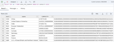
To make the results more interesting, we could generate the same report, but this time ordered by capacity per country size. To evaluate the size of a country, we can use spatial function
ST_Area.
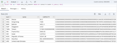
SELECT TOP 10 *
FROM CAPA_PER_COUNTRY
ORDER BY CAPACITY/SHAPE.ST_AREA() DESC
The result of this analysis looks significantly different.
We could have easily achieved the top list by capacity by just using the Global Power Plants dataset and without doing our spatial join. However, the last analysis (capacity per area) can only be done knowing the actual administrative boundaries.
Source: sap.com




No comments:
Post a Comment