After completing the first part of the blog you should have a hold-out dataset in HANA dedicated to test, for both the Census case, and the California Housing case. In this second part we will build an APL model and a non-APL model on the same training data. Predictions will be made against the hold-out dataset to ensure a fair comparison between the two models. We will use standard metrics to measure the accuracy of our classification models and our regression models.
Regression Use Case
from hana_ml import dataframe as hd
conn = hd.ConnectionContext(userkey='MLMDA_KEY')
target_col = 'Price'
key_col = 'Id'
# Sorted data for training
sql_cmd = 'SELECT * FROM "APL_SAMPLES"."HOUSING_TRAIN" ORDER BY 1'
train_remote = hd.DataFrame(conn, sql_cmd)
# Data for test without the known target
test_remote = conn.table('HOUSING_TEST', schema='APL_SAMPLES').drop([target_col])
We train an APL regression model on the train table, keeping the default parameters:
from hana_ml.algorithms.apl.gradient_boosting_regression import GradientBoostingRegressor
apl_model = GradientBoostingRegressor()
apl_model.fit(train_remote, label=target_col, key=key_col)
We make predictions using the hold-out dataset as recommended in the first part:
apl_pred_remote = apl_model.predict(test_remote).rename_columns(['ID', 'PREDICTED'])
apl_pred_remote.save(('HOUSING_APL_PREDICTIONS'), force = True)
We estimate the accuracy of the predictions with the MAE and RMSE indicators:
sql_cmd = """
select
round(avg(abs(P."PREDICTED" - A."Price")),4) as "Mean Absolute Error",
round(sqrt(avg(power(P."PREDICTED" - A."Price",2))),4) as "Root Mean Square Error"
from "USER_APL"."HOUSING_APL_PREDICTIONS" P, "APL_SAMPLES"."HOUSING_TEST" A
where P."ID" = A."Id"
"""
apl_err_remote = hd.DataFrame(conn, sql_cmd)
apl_err_remote.collect()
You may want to define a naïve regressor that will serve as a baseline; in the following example the predicted value is the mean price from the training dataset, and it is compared to the actual price in the test dataset:
sql_cmd = """
With
NAIVE as (
select avg("Price") as PREDICTED from "APL_SAMPLES"."HOUSING_TRAIN"
)
select
round(avg(abs(P."PREDICTED" - A."Price")),4) as "Mean Absolute Error",
round(sqrt(avg(power(P."PREDICTED" - A."Price",2))),4) as "Root Mean Square Error"
from NAIVE P, "APL_SAMPLES"."HOUSING_TEST" A
"""
naive_err_remote = hd.DataFrame(conn, sql_cmd)
naive_err_remote.collect()
As expected, the naïve regressor makes much larger errors than the APL regressor:
Now, let’s try the random forest technique from scikit-learn; again, we keep the default parameters:
# Learning
df_train = conn.table('HOUSING_TRAIN', schema='APL_SAMPLES').collect()
x_train = df_train.drop(columns=[target_col, key_col])
y_train = df_train[target_col]
from sklearn.ensemble import RandomForestRegressor
rdf_model = RandomForestRegressor()
rdf_model.fit(x_train, y_train)
# Make Predictions on hold-out
df_test = conn.table('HOUSING_TEST', schema='APL_SAMPLES').collect()
x_test = df_test.drop(columns=[target_col, key_col])
y_test = df_test[target_col]
rdf_pred_df = rdf_model.predict(x_test)
Here are the MAE and the RMSE values:
import numpy as np
# MAE
rdf_abs_err_df = abs(rdf_pred_df - y_test)
rdf_mae = np.mean(rdf_abs_err_df)
print('MAE : %.3f' % rdf_mae)
# RMSE
rdf_square_err_df = (rdf_pred_df - y_test)**2
rdf_rmse = np.sqrt(np.mean(rdf_square_err_df))
print('RMSE: %.3f' % rdf_rmse)
Our two trained models do much better than the mean price naïve approach. The APL gradient boosting model makes less errors than the random forest model; this comes with no surprise since gradient boosting trees are usually more accurate than random forests.
Classification Use Case
For building the APL classification model, we follow the same steps that we used in the regression case.
Step 1 – Define the HANA datafames:
target_col = 'class'
key_col = 'id'
# Sorted data for training
sql_cmd = 'SELECT * FROM "APL_SAMPLES"."CENSUS_TRAIN" ORDER BY 1'
train_remote = hd.DataFrame(conn, sql_cmd))
# Data for test without the known target
test_remote = conn.table('CENSUS_TEST', schema='APL_SAMPLES').drop([target_col])
Step 2 – APL model fit on the training data:
from hana_ml.algorithms.apl.gradient_boosting_classification import GradientBoostingBinaryClassifier
apl_model = GradientBoostingBinaryClassifier()
apl_model.fit(train_remote, label=target_col, key=key_col)
Step 3 – Predict the target using the hold-out data:
apl_model.set_params(extra_applyout_settings={'APL/ApplyExtraMode': 'AllProbabilities'})
apl_pred_remote = apl_model.predict(test_remote).rename_columns(['ID', 'PREDICTED', 'PROBA'])
Step 4 – Evaluate the accuracy of the predictions:
sql_cmd = """
select A."id", A."class" as ACTUAL, P."PREDICTED", P."PROBA"
from "USER_APL"."CENSUS_APL_PREDICTIONS" P, "APL_SAMPLES"."CENSUS_TEST" A
where P."ID" = A."id"
"""
apl_pred_remote = hd.DataFrame(conn, sql_cmd)
apl_pred_df = apl_pred_remote.collect()
For classification accuracy metrics we will leverage scikit-learn functions:
from sklearn.metrics import classification_report
import matplotlib.pyplot as plt
from sklearn.metrics import RocCurveDisplay
Here is a typical report to assess the accuracy of our APL classifier:
print(classification_report(
y_true=(apl_pred_df.ACTUAL==1),
y_pred=(apl_pred_df.PREDICTED==1)
))
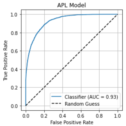
One can draw the ROC curve and display the AUC value:
RocCurveDisplay.from_predictions(
y_true=(apl_pred_df.ACTUAL==1),
y_pred=(apl_pred_df.PROBA)
)
plt.title('APL Model')
plt.plot([0, 1], [0, 1], "k--", label="Random Guess")
plt.axis("square")
plt.xlabel("False Positive Rate")
plt.ylabel("True Positive Rate")
plt.legend()
plt.grid()
plt.show()
To conclude, we will define a naïve classifier where the predicted class is the most frequent class from the training dataset ; it is compared to the actual class in the test dataset:
sql_cmd = """
With
NAIVE as (
select top 1 "class" as PREDICTED, count(*) as N
from "APL_SAMPLES"."CENSUS_TRAIN"
group by "class" order by 2 desc
)
select A."id", A."class" as ACTUAL, P."PREDICTED"
from NAIVE P, "APL_SAMPLES"."CENSUS_TEST" A
"""
naive_pred_remote = hd.DataFrame(conn, sql_cmd)
naive_pred_df = naive_pred_remote.collect()
To evaluate our naïve classifier we run the same report used earlier for APL:
print(classification_report(
y_true=(naive_pred_df.ACTUAL==1),
y_pred=(naive_pred_df.PREDICTED==1)
))
This naïve classifier predicts class 0 always, the most frequent class in the train dataset:
df_remote = conn.table('CENSUS_TRAIN', schema='APL_SAMPLES')
df = df_remote.agg([('count', 'class', 'rows')], group_by='class').collect()
df['Train percent'] = (df['rows'] / df['rows'].sum()) * 100
df.style.hide(axis='index')
The test dataset was built so that it preserves the distribution of the class:
df_remote = conn.table('CENSUS_TEST', schema='APL_SAMPLES')
df = df_remote.agg([('count', 'class', 'rows')], group_by='class').collect()
df['Test percent'] = (df['rows'] / df['rows'].sum()) * 100
df.style.hide(axis='index')
Our naive classifier makes a correct prediction 76-percent of the time.


No comments:
Post a Comment