I am writing this blog to show basic classification training procedures using python package hana_ml. Wtih class UnifiedClassification, you can use several classification algorithms. Besides, training result can be exported as HTML report easily.
Environment
Environment is as below.
◉ Python: 3.7.13(Google Colaboratory)
◉ HANA: Cloud Edition 2022.16
Python packages and their versions.
◉ hana_ml: 2.13.22072200
◉ pandas: 1.3.5
◉ scikit-learn: 1.0.2
As for HANA Cloud, I activated scriptserver and created my users. Though I don’t recognize other special configurations, I may miss something since our HANA Cloud was created long time before.
I didn’t use HDI here to make environment simple.
Generated Model Report
Firstly let me show you model report. A report can be displayed within jupyter or downloaded as html file. I didn’t optimize hyper-parameters, so there is no optimal parameter page.
The report is for training and validation, not for test.
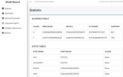
Statistic
Basic classification result is shown in Static page.
I don’t know much about KAPPA and MCC, Probably they are as below.
KAPPA: Cohen’s kappa
Parameter
Used parameters for classification.
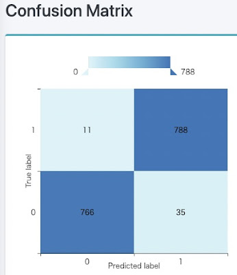
Confusion Matrix
Variables screen shows variable statistics.
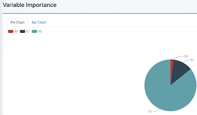
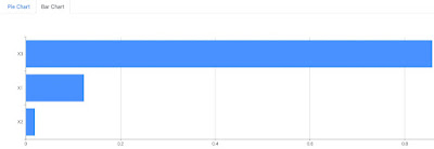
Variable Importance
Variable importance is visualized as pie chart or bar chart.
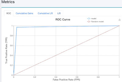
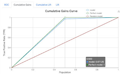
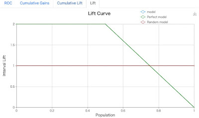
Metrics
24 types of metrics are exported.
Python Script
1. Install Python packages
Install python package hana_ml, which is not pre-installed on Google Colaboratory.
As for pandas and scikit-learn, I used pre-installed ones.
!pip install hana_ml
2. Import modules
Import python package modules.
from hana_ml.dataframe import ConnectionContext, create_dataframe_from_pandas
from hana_ml.algorithms.pal.partition import train_test_val_split
from hana_ml.algorithms.pal.unified_classification import UnifiedClassification
import pandas as pd
from sklearn.datasets import make_classification
3. Connect to HANA Cloud
Connect to HANA Cloud and check its version.
ConnectionContext class is for connection to HANA.
HOST = '<HANA HOST NAME>'
SCHEMA = USER = '<USER NAME>'
PASS = '<PASSWORD>'
conn = ConnectionContext(address=HOST, port=443, user=USER,
password=PASS, schema=SCHEMA)
print(conn.hana_version())
4.00.000.00.1660640318 (fa/CE2022.16)
4. Create test data
Create test data using scikit-learn.
There are 3 features and 1 target variable.
def make_df():
X, y = make_classification(n_samples=1000,
n_features=3, n_redundant=0)
df = pd.DataFrame(X, columns=['X1', 'X2', 'X3'])
df['CLASS'] = y
return df
df = make_df()
print(df)
df.info()
Here is dataframe overview.
X1 X2 X3 CLASS
0 0.964229 1.995667 0.244143 1
1 -1.358062 -0.254956 0.502890 0
2 1.732057 0.261251 -2.214177 1
3 -1.519878 1.023710 -0.262691 0
4 4.020262 1.381454 -1.582143 1
.. ... ... ... ...
995 -0.247950 0.500666 -0.219276 1
996 -1.918810 0.183850 -1.448264 0
997 -0.605083 -0.491902 1.889303 0
998 -0.742692 0.265878 -0.792163 0
999 2.189423 0.742682 -2.075825 1
[1000 rows x 4 columns]
<class 'pandas.core.frame.DataFrame'>
RangeIndex: 1000 entries, 0 to 999
Data columns (total 4 columns):
# Column Non-Null Count Dtype
--- ------ -------------- -----
0 X1 1000 non-null float64
1 X2 1000 non-null float64
2 X3 1000 non-null float64
3 CLASS 1000 non-null int64
dtypes: float64(3), int64(1)
memory usage: 31.4 KB
5. define table and upload data
Define HANA Table and upload data using function “create_dataframe_from_pandas”.
The function is very useful, since it automatically define table and upload at the same time. Please check options for further detail.
TRAIN_TABLE = 'PAL_TRAIN'
dfh = create_dataframe_from_pandas(conn, df, TRAIN_TABLE,
schema=SCHEMA,
force=True, # True: truncate and insert
replace=True) # True: Null is replaced by 0
6. Check upload result
check the result of HANA table definition and upload result. With HANA dataframe, python has connection to HANA table, so need to collect when getting data.
def show_hana_df(dfh):
print(dfh.collect())
print(f'Table Structure: {dfh.get_table_structure()}')
print(dfh.describe().collect())
show_hana_df(dfh)
X1 X2 X3 CLASS
0 0.964229 1.995667 0.244143 1
1 -1.358062 -0.254956 0.502890 0
2 1.732057 0.261251 -2.214177 1
3 -1.519878 1.023710 -0.262691 0
4 4.020262 1.381454 -1.582143 1
.. ... ... ... ...
995 -0.247950 0.500666 -0.219276 1
996 -1.918810 0.183850 -1.448264 0
997 -0.605083 -0.491902 1.889303 0
998 -0.742692 0.265878 -0.792163 0
999 2.189423 0.742682 -2.075825 1
[1000 rows x 4 columns]
Table Structure: {'X1': 'DOUBLE', 'X2': 'DOUBLE', 'X3': 'DOUBLE', 'CLASS': 'INT'}
column count unique nulls mean std min max \
0 X1 1000 1000 0 -0.022545 1.403956 -4.543441 4.020262
1 X2 1000 1000 0 0.006131 0.987222 -3.019512 3.926238
2 X3 1000 1000 0 -0.048433 1.322137 -3.836929 3.994644
3 CLASS 1000 2 0 0.498000 0.500246 0.000000 1.000000
median 25_percent_cont 25_percent_disc 50_percent_cont \
0 -0.197133 -1.054538 -1.056985 -0.197133
1 -0.000251 -0.648000 -0.649373 -0.000251
2 -0.224366 -1.021008 -1.021405 -0.224366
3 0.000000 0.000000 0.000000 0.000000
50_percent_disc 75_percent_cont 75_percent_disc
0 -0.197984 0.990549 0.990513
1 -0.000709 0.666021 0.665924
2 -0.229456 0.969732 0.967854
3 0.000000 1.000000 1.000000
7. Split data into train and test dataset
Split dataset using function “train_test_val_split”. The function needs key columns, so I added key column using function “add_id”.
train, test, _ = train_test_val_split(dfh.add_id(),
testing_percentage=0.2,
validation_percentage=0)
print(f'Train shape: {train.shape}, Test Shape: {test.shape}')
Train shape: [8000, 5], Test Shape: [2000, 5]
8. Training
Train with random forest by using class “UnifiedClassification”. When fitting I used partitioning for validation.
rdt_params = dict(n_estimators=10, max_depth=10)
uc_rdt = UnifiedClassification(func = 'RandomDecisionTree', **rdt_params)
uc_rdt.fit(data=train, training_percent=0.8, ntiles=2, key='ID',
partition_method='stratified', stratified_column='CLASS',
build_report=True)
9. Training result
9.1. Raw result
Raw result is in attribute “model_”.
for model in uc_rdt.model_:
print(model.collect(), '\n')
Third dataframe is empty, since I don’t optimize hyper parameters.
ROW_INDEX PART_INDEX MODEL_CONTENT
0 0 -1 <PMML version="4.0" xmlns="http://www.dmg.org/...
1 1 0 <PMML version="4.0" xmlns="http://www.dmg.org/...
2 2 0 " />\n<sd v="1" n="191" />\n<Node id="40" sc="...
-- ommision --
36 36 9 ode>\n<Node id="40" sc="0" n="76" >\n<sp x="X2...
37 37 9 "0" n="74" />\n<sd v="1" n="705" />\n<Node id=...
38 38 9 " op="lt" v="-0.476949" />\n<sd v="0" n="0" />...
STAT_NAME STAT_VALUE CLASS_NAME
0 AUC 0.97875 None
1 RECALL 0.9637046307884856 0
2 PRECISION 0.9935483870967742 0
3 F1_SCORE 0.9783989834815756 0
4 SUPPORT 799 0
5 RECALL 0.9937578027465668 1
6 PRECISION 0.9648484848484848 1
7 F1_SCORE 0.9790897908979089 1
8 SUPPORT 801 1
9 ACCURACY 0.97875 None
10 KAPPA 0.9574983397788976 None
11 MCC 0.9579295387997437 None
Empty DataFrame
Columns: [PARAM_NAME, INT_VALUE, DOUBLE_VALUE, STRING_VALUE]
Index: []
ACTUAL_CLASS PREDICTED_CLASS COUNT
0 0 0 770
1 0 1 29
2 1 0 5
3 1 1 796
VARIABLE_NAME IMPORTANCE
0 X1 0.125881
1 X2 0.018198
2 X3 0.855921
NAME X Y
0 RANDOM_CUMGAINS 0.0 0.00000
1 RANDOM_CUMGAINS 1.0 1.00000
2 RANDOM_LIFT 0.0 1.00000
3 RANDOM_LIFT 1.0 1.00000
4 RANDOM_CUMLIFT 0.0 1.00000
5 RANDOM_CUMLIFT 1.0 1.00000
6 PERF_CUMGAINS 0.0 0.00000
7 PERF_CUMGAINS 0.5 1.00000
8 PERF_CUMGAINS 1.0 1.00000
9 PERF_LIFT 0.0 2.00000
10 PERF_LIFT 0.5 2.00000
11 PERF_LIFT 1.0 0.00000
12 PERF_CUMLIFT 0.0 2.00000
13 PERF_CUMLIFT 0.5 2.00000
14 PERF_CUMLIFT 1.0 1.00000
15 ROC_FPR 0.0 0.00000
16 ROC_TPR 0.0 0.00000
17 ROC_FPR 1.0 0.02125
18 ROC_TPR 1.0 0.97875
19 ROC_FPR 2.0 1.00000
20 ROC_TPR 2.0 1.00000
21 CUMGAINS 0.0 0.00000
22 CUMGAINS 0.5 0.97875
23 CUMGAINS 1.0 1.00000
24 LIFT 0.0 2.00000
25 LIFT 0.5 1.00000
26 LIFT 1.0 0.00000
27 CUMLIFT 0.0 2.00000
28 CUMLIFT 0.5 1.95750
29 CUMLIFT 1.0 1.00000
9.2. Model report
Instance “UnifiedClassification” can generate model report.
“generate_notebook_iframe_report” function show a report in Jupyter.
“generate_html_report” function save a html report file. Its parameter is fine name prefix, so “result_unified_classification_model_report.html” is the complete fine name in this script.
uc_rdt.generate_notebook_iframe_report()
uc_rdt.generate_html_report('result')
10. Test
10.1. Scoring
With “score” function, you can get metrics.
results = uc_rdt.score(data=test, key='ID')
for result in results:
print(result.collect())
ID SCORE CONFIDENCE \
0 2 0 1.0
1 3 0 0.6
2 7 1 1.0
3 13 1 1.0
4 28 1 1.0
... ... ... ...
1995 9963 1 1.0
1996 9975 0 0.8
1997 9995 1 1.0
1998 9998 1 1.0
1999 10000 1 1.0
REASON_CODE
0 [{"attr":"X3","pct":98.0,"val":0.4868758174245...
1 [{"attr":"X1","pct":65.0,"val":0.3245506374878...
2 [{"attr":"X3","pct":78.0,"val":0.4052506627718...
3 [{"attr":"X3","pct":90.0,"val":0.4588332547405...
4 [{"attr":"X1","pct":74.0,"val":0.6337552163132...
... ...
1995 [{"attr":"X3","pct":91.0,"val":0.4566825270920...
1996 [{"attr":"X3","pct":88.0,"val":0.4430019995088...
1997 [{"attr":"X1","pct":76.0,"val":0.6453786485350...
1998 [{"attr":"X3","pct":85.0,"val":0.4241043164237...
1999 [{"attr":"X3","pct":88.0,"val":0.4362227541608...
[2000 rows x 4 columns]
STAT_NAME STAT_VALUE CLASS_NAME
0 AUC 0.99131975 None
1 RECALL 0.9710578842315369 0
2 PRECISION 0.9898270600203459 0
3 F1_SCORE 0.980352644836272 0
4 SUPPORT 1002 0
5 RECALL 0.9899799599198397 1
6 PRECISION 0.9714847590953786 1
7 F1_SCORE 0.9806451612903225 1
8 SUPPORT 998 1
9 ACCURACY 0.9805 None
10 KAPPA 0.9610013259549175 None
11 MCC 0.9611748218717623 None
ACTUAL_CLASS PREDICTED_CLASS COUNT
0 0 0 973
1 0 1 29
2 1 0 10
3 1 1 988
NAME X Y
0 RANDOM_CUMGAINS 0.00 0.000000
1 RANDOM_CUMGAINS 1.00 1.000000
2 RANDOM_LIFT 0.00 1.000000
3 RANDOM_LIFT 1.00 1.000000
4 RANDOM_CUMLIFT 0.00 1.000000
.. ... ... ...
141 CUMLIFT 0.80 1.246250
142 CUMLIFT 0.85 1.174118
143 CUMLIFT 0.90 1.109444
144 CUMLIFT 0.95 1.051579
145 CUMLIFT 1.00 1.000000
[146 rows x 3 columns]
10.2. prediction
If you want to get each prediction result, just call “predict” function.
df_pred = uc_rdt.predict(data=test, key='ID')
print(df_pred.collect())
ID SCORE CONFIDENCE \
0 2 0 1.0
1 3 0 0.6
2 7 1 1.0
3 13 1 1.0
4 28 1 1.0
... ... ... ...
1995 9963 1 1.0
1996 9975 0 0.8
1997 9995 1 1.0
1998 9998 1 1.0
1999 10000 1 1.0
REASON_CODE
0 [{"attr":"X3","pct":98.0,"val":0.4868758174245...
1 [{"attr":"X1","pct":65.0,"val":0.3245506374878...
2 [{"attr":"X3","pct":78.0,"val":0.4052506627718...
3 [{"attr":"X3","pct":90.0,"val":0.4588332547405...
4 [{"attr":"X1","pct":74.0,"val":0.6337552163132...
... ...
1995 [{"attr":"X3","pct":91.0,"val":0.4566825270920...
1996 [{"attr":"X3","pct":88.0,"val":0.4430019995088...
1997 [{"attr":"X1","pct":76.0,"val":0.6453786485350...
1998 [{"attr":"X3","pct":85.0,"val":0.4241043164237...
1999 [{"attr":"X3","pct":88.0,"val":0.4362227541608...
[2000 rows x 4 columns]
11. Close connection
Last but not least, closing connection explicitly is preferable.
conn.close()



No comments:
Post a Comment