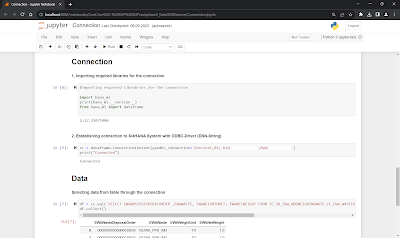
After connecting an SAP S/4HANA System with Python and Jupyter Notebook using an ODBC driver we can now work with the data we retrieved.
In the world of data science, detecting anomalies and errors is an essential task. In this blog, we will explore a data science project (from my practical phase in my dual curriculum) focusing on detecting implausible, manually-entered weighing notes where for example the weighing unit was mixed up. These anomalies can have significant consequences in inventory, billing, or logistics.
I will also use the CRISP-DM (Cross-Industry Standard Process for Data Mining) methodology which will guide guiding us through the various phases of the project: Business Understanding, Data Understanding, Data Preparation, Modeling, Evaluation, and Deployment. Each phase is a critical step towards building a robust anomaly detection system.
1. Business Understanding:
A vital step in any data science project is to gain a deep understanding in the business context of the problem at hand. In our case, the challenge lies in identifying such weighing notes that were entered manually by end users and that appear to be implausible. Example is a wrongly selected unit while manually entering the weight with the wrong amount. Such weighing notes may contain errors or inconsistencies, which can lead to inaccurate customer invoices, inaccurate data analysis, inaccurate decision-making, and operational disruptions.
2. Data Understanding:
To tackle this problem, we need to gather and analyze the relevant data. This includes exploring the structure of the manually entered weighing notes, identifying missing values, and gaining insights into potential data quality issues.
I asked experts where I could find the data, which specific data I needed and whether I had access to the data or not. In my case I wanted to access the data through Python and Jupyter. To make the connection between the S/4HANA System and Python / Jupyter I used an ODBC-Driver.
There, it is mentioned that we had to create a CDS (Core Data Services) View, a Service Definition, and a Service Binding to access the data.
Moreover, I used several Python libraries like Seaborn to visualize the data which can help us detect possible outliers without using outlier detection algorithms. By examining the structure, quality, and completeness of the data, we can gain knowledge about challenges we might encounter during the analysis phase.
In this example I used a boxplot to visualize the data which can provide insights into its central tendency, spread, and potential outliers.
# data
df_netweight_kg = cc.sql('SELECT EWAWASTEDISPOSALORDER, EWAWEIGHTUNIT, EWANETWEIGHT FROM ZC_SB_EWA_WDOWEIGHINGNOTE.ZC_EWA_WASTEORDERWEIGHINGNOTE WHERE EWANETWEIGHT <> 0 AND EWAWeightUnit = \'KG\'')
df_netweight_kg.collect()
# create a Pandas DataFrame
dff_netweight_kg = pd.DataFrame(df_netweight_kg.collect())
#BOXPLOT (unit TO)
boxplot_nw_to = dff_nw_to.boxplot(column='EWANetWeight',figsize = (7,5))
boxplot_nw_to.set_ylabel('Weight in TO')
boxplot_nw_to.set_xlabel('')
I got the following boxplot as a result:
In the boxplot we can clearly see 3 data points that could be considered outliers. This will be confirmed or denied with the result of the outlier detection methods.
3. Data Preparation:
Data preparation involves cleaning and transforming the data to the data to make it ready for analysis. Here we can focus on handling missing values, outliers, and inconsistencies in the weighing notes. Python’s data manipulation libraries, such as Pandas, are instrumental in this phase.
4. Modeling:
The modeling phase involves developing and implementing algorithms or models to detect implausible weighing notes. One powerful approach is the z-score technique, which identifies outliers by counting how many standard deviations you are away from the mean of your data. A z-score of 0 means the data point is on the mean, a higher score indicates the data point is higher than the mean and therefore, an outlier.
# Z score
from scipy import stats
import numpy as np
z = np.abs(stats.zscore(dff['EWANetWeight']))
#print(z)
mean = np.mean(dff['EWANetWeight'])
print("------------------------------------------------------------------------------------------")
print("Mean:", mean)
median = np.median(dff['EWANetWeight'])
print("------------------------------------------------------------------------------------------")
print("Median", median)
# threshold 2 gives the same outliers
threshold = 3
#position of the outlier
outlier_result = np.where(z > 2)
outlier_array = outlier_result[0]
print("------------------------------------------------------------------------------------------")
print(outlier_array)
# printing columns with given indexes/position
# Using the operator .iloc[] to select multiple rows
result = dff.iloc[outlier_array]
print("------------------------------------------------------------------------------------------")
print("Outliers: ")
display(result)
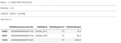
We implement this algorithm using the NumPy and SciPy library in Python.
With this method we get the following result:
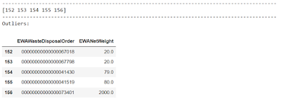
Another technique we used was the Inter Decile Range (IDR), which can detect outliers by calculating the range/distance between the first (10%) and ninth (90%) percentiles.
We used the NumPy library in Python for the implementation of this algorithm.
import pandas as pd
# IDR
#INTER DECILE RANGE
Q1 = np.percentile(net_weight , 10)
Q3 = np.percentile(net_weight, 90)
# Find IQR, upper limit, lower limit
IQR = Q3 - Q1
ul = Q3+1.5*IQR
ll = Q1-1.5*IQR
#position of the outlier
outlier_res = np.where((dff1['EWANetWeight'] > ul) | (dff1['EWANetWeight'] < ll))
outlier_array = outlier_res[0]
print("------------------------------------------------------------------------------------------")
print(outlier_array)
# Using the operator .iloc[] to select multiple rows
result = dff1.iloc[outlier_array]
print("------------------------------------------------------------------------------------------")
print ("Outliers: ")
display(result)
With the method IDR we get the following result:
5. Evaluation:
Once the models have been implemented it is crucial to evaluate the model’s performance. This involves measuring their performance by comparing its predictions against known anomalies. Approaches such as visual inspection, accuracy, precision, recall, or F1-score offer insight on the effectiveness of the model.
In this case, I chose the visual comparison. By comparing the boxplot, we created above with the result of the outlier methods we can see that the boxplot shows three data points that might be outliers: 2000 tones and two points close to 100 tones. The z-score method delivers us the outliers 2000 tones, 79 tones and 80 tones and the method IDR gives us the outliers 20 tones, 79 tones, 80 tones and 2000 tones. That shows us that the z-score method had the best performance out if the two outlier methods I chose.
By comparing different models and selecting the most suitable one, we can ensure the detection of implausible weighing notes with high accuracy. Here, we would select the z-score method because this methos had the best evaluation using visual comparison.
In my case the boxplot clearly showed possible outliers which I used for the comparison, but that might not always be the case. If you have a different data distribution you might want to consider other visualization methods and other evaluation approaches like the ones I mentioned above.
6. Deployment and maintenance:
The final stage of the CRISP-DM methodology is the deployment of the solution. We can integrate the trained model into the SAP S/4HANA on-premise system, enabling real-time anomaly detection as customers enter weighing notes or we can simply make sure that the data scientists of our customers get the outlier results so they dive deeper into the problem. Furthermore, regular model updates and maintenance are essential to adapt to evolving data patterns and maintain accuracy.
I haven’t integrated the model into the SAP system because in this blog I chose to focus on showing how to use the tools we have in python but the future goal is to deliver the outlier results to the data scientist so they can take a closer look at their data.


No comments:
Post a Comment