Calculation View In SAP HANA

Introduction

SAP HANA, or “High-Performance Analytic Appliance,” refers to a database management system and application platform that uses in-memory technology. SAP HANA is a well-liked option for businesses looking to speed up their decision-making processes because it is built to manage enormous volumes of data and perform real-time data processing and analytics.

First, let’s see what’s a view in general

A view is a kind of imaginary table that will have the results linked to the SQL statement. Note that the data from the SQL query need not come from a common database table.

In this blog, we’ll be learning the key aspects of graphical views in HANA.

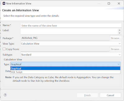
To create a graphical view, Right click on your package and select a new calc view

Choose the necessary option based on the requirements

Here you can choose between graphical and SQL view based on your interest

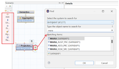
You can find all the required nodes from the Bucket listed on the left. To add a data source to the node. Click the + symbol on the node and search for the necessary table.

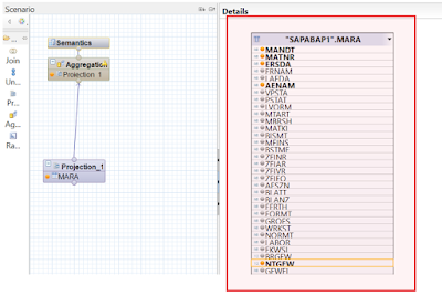
You can select the required fields from the table by just clicking on it

Kudos, that’s a simple Graphical view.

Now Let’s Go deep into the nodes available in the Calculation View

Join Node:

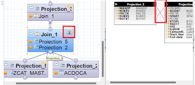
A join node is used to establish a relationship between 2 tables in HANA, and there are many types of join available in HANA. The most widely used are mentioned below

1. Inner join

2. Left outer join

3. Right outer join

Inner join

The inner join works similarly to the equation A ∩ B, Only common data between the 2 tables are considered.

OUTPUT

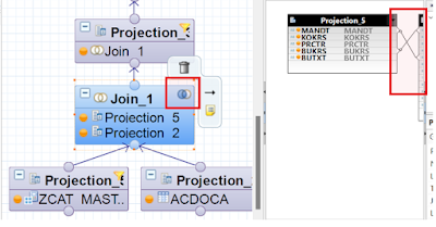
Here we are joining the Client(MANDT) and Company code(BUKRS) of ACDOCA and a Custom table. Thus the result of this view will only have the common company code and client from both tables.

Left Outer join

In the Left outer join all the data in the Primary table are considered and only the Common data in the transaction table will be propagated.

OUTPUT

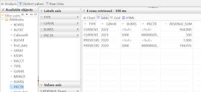
Here we are joining the Client(MANDT) and Company code(BUKRS) of ACDOCA and a Custom table. Thus the result of this view will have all the data from the primary table and common also the common data from the secondary table will be present in the output

The Null value in the below screenshot denotes that we have excess data from the left table that are not part of our requirement but they are passed since there happened to be a left outer join

Right Outer Join

In the Right outer join all the data in the Transaction table are considered and only the Common data in the master table will be propagated.

OUTPUT

Here we are joining the Client(MANDT) and Company code(BUKRS) of ACDOCA and a Custom table. Thus the result of this view will have all the data from the right table and the common data from the secondary table will be present in the output

The Null value in the below screenshot denotes that we have excess data from the right table that are not part of our requirement but they are passed since there happened to be a right outer join.

Union Node:

The union node is used to club/Combine the similar columns of 2 more Tables.

For Example, let’s assume 2 simple tables and apply union and check what happens to them.

The union will identify similar columns from different tables by comparing the header text and combining it as a single column.

If there are any duplicate entries, then the measure in the entry will get Summed up.

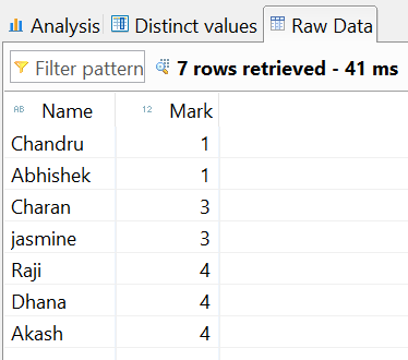
OUTPUT

You can see that the mark of ‘RAJI’ = 4 which is the sum of marks from TABLE 1 and TABLE 2

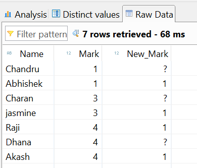
When you add a new entry to any of the tables, then the output will be something like the below, then the other tables that don’t have the column will contain a null value or ‘?’

Rank and Aggregation node

Now let’s change our gear and move to the Rank node and aggregation, The rank node helps us to sort the data in the table in Ascending or descending order, and we can set the threshold as per our requirement.

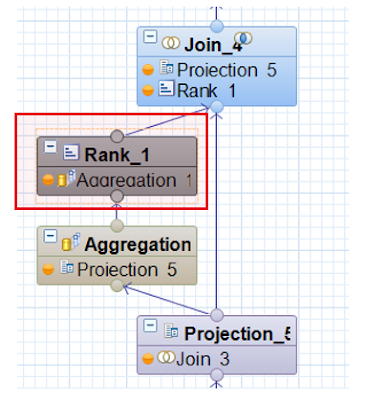
The above view is an example of calculating the top 5 revenue from projection 5

In projection 5 we have all the fields that we need. But we are only taking the necessary field to rank nodes. The aggregation node below the rank node is used to sum up the revenue with a common key hence we can get the revenue sorted in the desired order without any discrepancies.

To rank the top 5 revenue in descending order we are giving the threshold as 5, Order by as our aggregated rank column, and our Partition by as a dummy column which contains ‘A’

Output from rank node:

Projection Node:

The projection node is used to add new tables or views. It is also the place where we can specify new calculation columns and filter expression

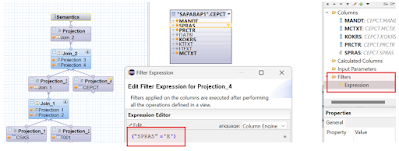
Giving a filter expression in the Projection view

We have CEPCT table to get the Profit centre and profit centre text(PRCTR and MCTXT). But we don’t need the profit centres that are not named in English. Hence we are applying a filter to SPARS(Language) field.

Now let’s see how to create a calculation column

A calculation column is the field whose values are based on the SQL expression which can have the name of other column values or Input parameters.

In the above example, we are creating a calculation column called Gross margin which is the result of the difference between Revenue and Actual Cost. The data type is mentioned as an integer.