The new Jupyter operator brings interactive Python Notebooks into your SAP Data Intelligence pipelines. Script your notebook directly in the pipeline and deploy exactly the same notebook and pipeline into production. No need to script in one place and to copy / paste the code into a Python operator.
Learn how to use the operator with a Machine Learning example, that forecasts multiple time-series in SAP HANA using the embedded Automated Predictive Library.
With Python you can implement a million things, other than Machine Learning by the way. Data retrieval or data preparation or just two further uses cases.
Prerequisites
The Jupyter operator was released in the first quarter of 2021 with SAP Data Intelligence Cloud, version 2013. Currently (April 2021) this functionality is not available in the on-premise release.
To implement the code in this blog, you also need to have access to a SAP HANA environment, which has the Automated Predictive Library installed. The trial of SAP HANA Cloud currently does not include that Automated Machine Learning library.
This hands-on tutorial assumes you are already familiar with both Jupyter notebooks and running basic graphs (which are also called pipelines) in SAP Data Intelligence. If you are new to the tool, you might benefit from the “Get Started” portal.
Introductory example – Execute once
Let’s keep it simple at first, with a very basic example. Use the Jupyter operator to send a signal every few seconds.
Open the “Modeler” and create a new, blank graph. Drag the Jupyter operator onto the canvas and give to it an “Output Port”, named “out”, of basic type “string”. Connect the output port with a Wiretap operator.
In order to open a Jupyter notebook to script in Python:
◉ You must specify a name for the notebook in the operator’s settings. The operator will create the notebook for you. If the pipeline is used in a Machine Learning scenario, you can also provide the name of a notebook that has already been created in the Machine Learning scenario.
◉ The Jupyter operator also has to be in none-Productive mode. This is the default setting, more on this later.
◉ The pipeline has to be running!
Set the “Notebook File Path” to: ping. Then save and run the pipeline.
With the pipeline running, you can now open the operator’s User Interface, the notebook.
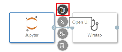
The notebook contains a lot of sample code, which gives a good introduction. Have a read, but eventually delete all content / cells to continue with the next steps.
Enter this code into a cell. Save the notebook and run the cell.
from datetime import datetime
now = datetime.now()
current_time = now.strftime('%H:%M:%S')
api.send('out', 'Ping @ ' + current_time)
Look into the Wiretap and you will see the time of your SAP Data Intelligence Cloud environment.
Introductory example – Responding to input port
Now change the pipeline, so that the Jupyter operator responds to data received on an input port. Stop the running pipeline and add an “Input Port”, named “in”, of basic type “string” to the Jupyter operator. Also add a “Constant Generator” in front, and set its mode to pulse, so that it sends a string every second.
Save and run the pipeline again. Open the Jupyter Operator’s UI as before. Replace the existing code with:
from datetime import datetime
def on_data_in(value):
now = datetime.now()
current_time = now.strftime('%H:%M:%S')
api.send('out', value + ' @ ' + current_time)
api.set_port_callback('in', on_data_in)
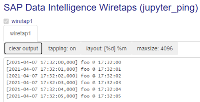
Remember so save the notebook and execute the cell. The Wiretap is now receiving and outputting the time every second.
Introductory example – Deploy
You can now script and execute the code. But how to run the code automatically, without you having to execute the code manually?
◉ The cells that should be executed without user intervention must be flagged as “productive”
◉ And the Jupyter operator’s status has to be switched to Productive
This approach allows you to keep code in your notebook that is not required for productive use. For instance keep any testing code in the notebook, just don’t flag it as “productive”.
While the pipeline is still running (with the default of “Productive” set to “False”), select the cell and click “Mark cell as productive”. This adds the “productive” tag to the cell. Save the notebook.
To run that code without your own intervention, stop the pipeline and change the Jupyter operator’s “Productive” status to “True”. Save and start the pipeline.
Now in productive mode the notebook cannot be opened anymore, as the code is supposed to run without manual intervention. SAP Data Intelligence automatically runs the cells that are flagged as productive. You can verify this by looking into the Wiretap. The Jupyter operator is sending the time every second on its own now.
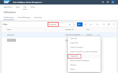
By the way, the Notebooks is saved on the file system of SAP Data Intelligence. You can see the exact location by searching for the notebook’s name in the System Management’s “Files” tab.
Introductory example – Forecast multiple time-series
At this point you are familiar with how the Jupyter operator works. Now use it to forecast multiple time-series. Time-series forecasting can be used for many different purposes, from demand forecasting to financial planning. You will use SAP HANA’s Automated Predictive Library to forecast the daily number of vehicles that are driving by various locations in the city of Zurich. The city has a number of automated counters installed and provides the numbers on their
Open Data portal (German speaking only)
Data upload
Download the file
VEHICLECOUNT.txt and upload it as table to SAP HANA. I prefer to use Python and the
hana_ml library for this uploading step. Below is the code needed when running the code in a Jupyter Notebook of a Machine Learning Scenario in SAP Data Intelligence.
Load the data into a pandas DataFrame. Note that the column that contains the month has to be converted into a Timestamp type. This example assumes that a SAP Data Intelligence already has a connection called ‘MYHANA’ to the SAP HANA system.
# Load CSV file into a pandas DataFrame
import pandas as pd
df_data = pd.read_csv("VEHICLECOUNT.txt", sep=";")
df_data.DATE= pd.to_datetime(df_data.DATE)
# Establish a connection from Python to SAP HANA
import hana_ml.dataframe as dataframe
from notebook_hana_connector.notebook_hana_connector import NotebookConnectionContext
conn = NotebookConnectionContext(connectionId = 'MYHANA')
# Create and upload into the table VEHICLECOUNT
df_remote = dataframe.create_dataframe_from_pandas(connection_context = conn,
pandas_df = df_data,
table_name = 'VEHICLECOUNT',
drop_exist_tab = True,
force = True)
DockerFile
The Jupyter operator already has a version of the
hana_ml library installed. However, for the time-series forecasting I want to use a newer version than the one that currently comes out of the box (April 2021).
Just go to the Repository tab and create a new DockerFile that installs the necessary version.
FROM $com.sap.sles.jupyter
RUN pip3.6 install --user hana-ml==2.6.21012600
Add the tag jupyter_hana_ml and build the DockerFile.

Time-series forecasting
Now to the real thing, the forecasting:
◉ In the modeler, create a new graph / pipeline. Add the Jupyter operator.
◉ Specify a name for the notebook: time_series_apl
◉ Place the Jupyter operator in a group, and assign the jupyter_hana_ml tag to the group
Now the Python code in the operator’s Notebook uses the hana_ml version installed in the DockerFile
As quick test, save and run the pipeline. Open the notebook’s UI, Delete all existing cells and check the hana_ml version with the code below. In case you see a warning about an lzma module, you can safely ignore it. Also mark the cell as productive, as it will be required when running the pipeline unsupervised.
import hana_ml
print(hana_ml.__version__)

Establish a connection to SAP HANA, using an existing connection from SAP Data Intelligence. Flag the cell as productive.
import hana_ml.dataframe as dataframe
from notebook_hana_connector.notebook_hana_connector import NotebookConnectionContext
conn = NotebookConnectionContext(connectionId = 'MYHANA')
Obtain a list of the locations where the cars are counted. These are the individual time-series / segments that will be forecasted. Flag the code as productive.
df_remote = conn.table("VEHICLEREG_APL")
segments = df_remote.select("COUNTRY").distinct().sort("COUNTRY", desc = False).collect()
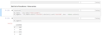
Display the locations / segments that were found. This code does not have to be flagged as productive.
segments
Before creating and saving new forecasts, drop old forecasts from the target table, if it exists. Flag the cell as productive.
from hdbcli import dbapi
dbapi_cursor = conn.connection.cursor()
if conn.sql("SELECT TABLE_OID FROM SYS.TABLES WHERE TABLE_NAME = 'VEHICLECOUNT_FORECASTS_SEGMENTED';").count() > 0:
dbapi_cursor.execute("""TRUNCATE TABLE VEHICLECOUNT_FORECASTS_SEGMENTED;""")
Create a pandas DataFrame to the store quality indicators of the created time-series. We will store for each time-series the Mean Absolute Percentage Error (MAPE). Flag this code as productive.
import pandas as pd
columns = ["SEGMENT", "MAPE"]
df_allmapes = pd.DataFrame(columns=columns)
Trigger the time-series forecasting. For each time-series, retrieve the individual history (from April 2020 to mid March 2021) and predict the daily number of vehicles for the following 7 days. The forecasts are created by the Automated Predictive Library, which is also used in SAP Analytics Cloud.
The predictions are written into the target table VEHICLECOUNT_FORECASTS_SEGMENTED, whilst the pandas DataFrame keeps track of the model quality of all time-series. Also flag this cell as productive.
from hana_ml.algorithms.apl.time_series import AutoTimeSeries
for index, row in df_segments.iterrows():
# Get raw data of each country
segment = row['LOCATION']
df_remote_segment = conn.sql("SELECT DATE, VEHICLECOUNT FROM VEHICLECOUNT WHERE LOCATION = '" + segment + "'")
# Sort data ascending, a requirement of the Automated Predictive Library
df_remote_segment = df_remote_segment.sort("DATE", desc = False)
# Forecast
tsapl = AutoTimeSeries(time_column_name = 'DATE', target = 'VEHICLECOUNT', horizon = 7)
tsapl.fit(data = df_remote_segment)
df_remote_aplforecast = tsapl.forecast(forecast_length = 7)
df_remote_aplforecast = df_remote_aplforecast.select('*', ("'" + segment + "'", 'SEGMENT'))
df_remote_aplforecast = df_remote_aplforecast.cast("SEGMENT", "NVARCHAR(100)") # Needed to ensure future segments with longer names can be stored
df_remote_aplforecast.save("VEHICLECOUNT_FORECASTS_SEGMENTED", append = True)
# Track model quality
ts_mape = tsapl.get_performance_metrics()['MAPE'][0]
df_allmapes = df_allmapes.append({"SEGMENT": segment, "MAPE": ts_mape}, ignore_index=True)
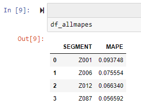
Running this cell will take a minute or two. When complete, display the collection of MAPEs. This cell is not required for productive use.
df_allmapes
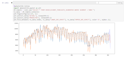
Plot the history and prediction of a single time-series. This cell also is not required for productive use.
%matplotlib inline
import matplotlib.pyplot as plt
df_remote = conn.sql("SELECT * FROM VEHICLECOUNT_FORECASTS_SEGMENTED WHERE SEGMENT ='Z001'")
ts_data = df_remote.collect()
plt.figure(figsize=(15, 5))
plt.plot(ts_data["ACTUAL"], linewidth=1)
plt.plot(ts_data["PREDICTED"], linewidth=1)
plt.fill_between( ts_data.index, ts_data["LOWER_INT_95PCT"], ts_data["UPPER_INT_95PCT"], color='b', alpha=.1);
The blue line represents the actual, known history. The orange line represents the predictions of the model. Towards the right you see how the model estimates the future pattern, for the 7 days following the known history. In case you know Zurich, the counter ‘Z001’ is at Strandbad Wollishofen, a road at lake Zurich that leads into town.
Save the notebook and pipeline.
Deployment
Everything is in place, to deploy the pipeline. In productive mode it would already drop previous predictions from the target table and fill it with the latest predictions.
We will just extend the graph a little, so that the Jupyter operator passes the collection of MAPEs to the output port, for further processing. Let’s send an email to the Administrator with information about the forecasts. Similarly, the information could be saved to SAP HANA or even directly to SAP Analytics Cloud for monitoring and analysis.
Stop the pipeline. Add an “Output Port” to the Jupyter operator, named “out”, of basic type “string”. Add a few more operators.
◉ A “Blank JS Operator” with an input port called in, and an output port called out. Both of basic type string. This operator will retrieve the collection of MAPEs and prepare the content of the email.
◉ Add a “Send Email” operator, if you have an SMTP Server available to you. If not, you could replace this operator with a Wiretap.
◉ Followed by a “Graph Terminator”.

Add this code to the “Blank JS Operator”
$.setPortCallback("in", writeEmail)
function writeEmail(ctx, data) {
all_mapes = JSON.parse(data);
ts_count = Object.keys(all_mapes).length
var email_body = "Hello,\nThe new forecasts have been created.\
\n\
\nNumber of forecasts: " + ts_count + "\
\nForecast with the lowest MAPE: " + (all_mapes[0].MAPE * 100).toFixed(1) + "% - " + all_mapes[0].SEGMENT +"\
\nForecast with the highest MAPE: " + (all_mapes[ts_count - 1].MAPE * 100).toFixed(1) + "% - " + all_mapes[ts_count -1].SEGMENT +"\
\n\
\nAll the best,\
\nYour SAP Data Intelligence system"
email_content = {"Attributes" : {"email.from" : "your@email.com",
"email.subject": "Forecast notification"},
"Body": email_body }
$.out(email_content);
}
Configure the “Send Email” operator by adding your SMTP server details into the operator’s connection. Also specify a recipient’s email address in the “Default To value” option.
Now just add the code to the Notebook, that passes the collection of MAPEs to the output port. Start the pipeline to be able to open the Jupyter notebook. The operator should have the “Productive” flag still set to “False”.
Open the notebook and add these lines. Flag the cell as productive and save the notebook. You can run the cell, but this will trigger the subsequent operators, including the “Graph Terminator”. Be careful, as once the graph is terminated, you cannot use the notebook anymore and you might lose unsaved changes.
df_allmapes = df_allmapes.sort_values(by = 'MAPE')
api.send("out", df_allmapes.to_json(orient = 'records'))
Best save the notebook and pipeline. Stop the pipeline. Set the Jupyter operator to “Productive” and run the pipeline again. The pipeline should now:
◉ run for a few minutes
◉ create and write the forecasts to SAP HANA
◉ send an email notification
◉ shut down
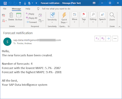
Schedule this pipeline and your forecasts will stay up to date.


No comments:
Post a Comment